The following function below allows you to get the number of visible rows from a filtered sets of rows in Excel using VBA. The function takes two arguments which is the Column and StartRow. Calling the FilterCount() function returns the number of visible rows. Also added an error handler which process the error description to determine if there's a visible row.
Parameters: Column:The column of the data to be filtered. If you have multiple columns being filtered you can just set the first Column or any column in the dataset. StartRow:Start row of the data to be filtered.
Function FilterCount(ByVal Column As String, ByVal StartRow As Long) As Long
You might be working on a project where you need to filter sets of data and create a raw data of that filtered sets of data to a new sheet or range.
By default, Excel copies hidden or filtered cells in addition to visible cells. If some cells, rows, or columns on your worksheet are not displayed, you have the option of copying all cells or only the visible cells.
The following snippet allows you to automate the process in microseconds.
[VBA]
Public Function GetFilteredData()
    Dim rawWs As Worksheet            'RAW DATA WORKSHEET
    Dim tarWs As Worksheet            'TARGET WORKSHEET

    'Replace this with your actual Worksheets
    Set rawWs = Sheets("Raw Data")
    Set tarWs = Sheets("Filtered Data Visualizations")

    Application.ScreenUpdating = False

    'Clear old contents of the Target Worksheet
    tarWs.Range("A2:N" & Rows.Count).ClearContents

    '****************************************************
    ' Select Raw Data Sheet and
    ' Copy only the visible rows if filter is applied
    '
    rawWs.Select
    Range("A2", Cells(ActiveSheet.UsedRange.Rows.Count, Range("N2").Column)).SpecialCells(xlCellTypeVisible).Copy

    '****************************************************
    'Select the Target worksheet and
    'Paste the copied data
    '
    tarWs.Select
    Range("A2").Select
    ActiveSheet.Paste
    Application.CutCopyMode = False

    Range("A2").Select
    Application.ScreenUpdating = True
End Function
'Set the range of all visible cells of the filtered data Set rngF = Range("A2", Cells(ActiveSheet.UsedRange.Rows.Count, _ Range("A2").Column)).SpecialCells(xlCellTypeVisible)
For Each Rng In Range("$A2:$A$" & lRow) If Not Intersect(Rng, rngF) Is Nothing Then If rngVal Is Nothing Then Set rngVal = Rng Else Set rngVal = Union(rngVal, Rng) End If If rngVal.Cells.Count = lRow Then Exit For End If Next Rng
'Resize array variable ReDim FilteredRows(0 To Application.CountA(rngVal)) As Variant
For Each val In rngVal If RowPrefixed = True Then FilteredRows(i) = val.Address Else FilteredRows(i) = Split(val.Address, "$")(2) End If
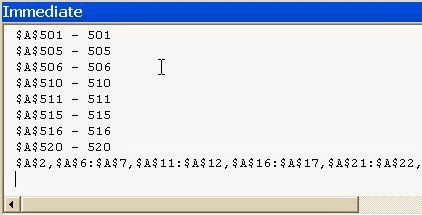
Debug.Print val.Address & " - " & Split(val.Address, "$")(2) i = i + 1 Next val
Debug.Print rngVal.Address
Applicaiton.ScreenUpdating = True End Function
To use the above function, you can assigned the following macro to a button or shape.
Sub SetFilter()
    Call GetFilteredRows(True)
End Sub
And you can see the output in the Immediate window as shown below.
In Microsoft Excel, you can suppress the message warning and alerts especially when you try to create a copy of a worksheet from a workbook containing macros to a new workbook which you wanted to save it as .xls or .xlsx extensions. By that, when you save the document it will prompt you to whether save the work as macro-enabled or macro-free workbook.
You can do that by setting DisplayAlerts to False with VBA code.
You might be creating templates with Microsoft Excel, and one of the feature you want is add a check boxes control where users can choose their option.
We'll, if you want to have another look aside from the default check box control. You can still create and customize your check box controls with a little VBA code to get it done.
In this example, I have here choices for the reason of a leave application form. I make use of the Microsoft Excel's Cell as a check box. It's just a matter of resizing the rows and columns to make the size of the cell equal.
1.) Now, let's create first the list of choices, as you can see below I've resized the cells and add borders on the cells which we'll set as a check-cell box control.
2.) Right Click on the Worksheet, then Click "View Code". 3.) Then Copy and Paste the following codes below into the code editor window.
The following code will set the Target Range of when the Check-Cell box will be triggered. I set the columns to G & H or it's numeric equivalent 7 & 8. Then create case statement of what rows it will run. The columns and rows may vary depending on your actual template. So you can set it to match your template.
Private Sub Worksheet_SelectionChange(ByVal Target As Range)
    With Target
        'SET THE TARGET COLUMN TO COLUMNS 7 AND 8
        If Target.Column >= 7 And Target.Column <= 8 Then
            'SELECT CASE OF WHAT ROW WILL BE SELECTED
            Select Case Target.Row
                Case 19 'SICK LEAVE
                    CheckSelected 19, 7
                Case 21 'VACATION LEAVE
                    CheckSelected 21, 7
                Case 23 'PERSONAL
                    CheckSelected 23, 7
                Case 25 'EMERGENCY
                    CheckSelected 25, 7
                Case 27 'APPOINTMENT
                    CheckSelected 27, 7
                Case 29 'OTHERS
                    CheckSelected 29, 7
                Case Default
            End Select
        End If
    End With
End Sub


'CHECK IF THE REASON IS CURRENTLY SELECTED
Sub CheckSelected(Row As Integer, Col As Integer)
    With Cells(Row, Col)
        If .Value = "+" Then
            .Value = ""
            ResetSelectedColor Row, Col
        Else
            .Value = "+"
            ApplySelectedColor Row, Col
        End If
    End With
End Sub


'CHANGE THE BACKGROUND OF THE SELECTION
Sub ApplySelectedColor(Row As Integer, Col As Integer)
    With Cells(Row, Col).Interior
        .Pattern = xlSolid
        .PatternColorIndex = xlAutomatic
        .ThemeColor = xlThemeColorAccent1
        .TintAndShade = 0.599993896298105
        .PatternTintAndShade = 0
    End With
End Sub


'REMOVE THE BACKGROUND OF THE SELECTION
Sub ResetSelectedColor(Row As Integer, Col As Integer)
    With Cells(Row, Col).Interior
        .Pattern = xlNone
        .TintAndShade = 0
        .PatternTintAndShade = 0
    End With
End Sub
4.) Now, if you select the Cells it should change the background with the "+" value. You may also change the value to whatever you want.
Named Ranges in Excel enable you to give one, or a group of cells a name other than the default B4 for a single cell, or B2:E20 for a range of cells. So that you can refer to them in formulas using that name.
When using Named Ranges there are also set of rules which you need to know like the scope where you can use the specified named range. If it's within only a single worksheet or the entire workbook.
Check this out Named Range Rules and be totally aware of the do's and don'ts when using this functions.
Managing Your Named Ranges There'll come a time when you want to edit or delete a Named Range. To do this access the Name Manager on the Formulas tab of the ribbon. The Name Manager Dialog box will open.
From here you can Edit and Delete your Named Ranges, or even create new ones. Remember, once you delete a name you cannot undo that action.
Different uses for Named Ranges in Excel: 1) Formula References: Simplify the creation and retrospective interpretation of formulas by using Named Ranges in your formulas
2) Multiple Print Areas on one worksheet; Selecting non-contiguous print areas is quick and easy using Named Ranges. Note: Excel 2007 onward allows you to set multiple print areas on the Page Layout Tab of the Ribbon under Print Area.
3) Reduce worksheet clutter with Named Constants. Sounds complicated but it's not. A Named Constant is just a fancy name given to values you might use repeatedly in your formulas. For example, let's say you're planning to have a year-end inventory sale and wanted to give a 10% discount on selected products, you could give the value "10%" a name like "Discount" and then you could:
Write your formulas like this =C1-(C1*Discount). This is more intuitive when you come to review the spreadsheet later, or for anyone else reviewing it.
Update the value globally by editing it once in the Name Manager. This will then automatically update the formulas.
Reduce clutter on your spreadsheet. Often a helper cell is set up with this key figure in to achieve these benefits, but if you've got many of these key figures your spreadsheets can become crowded.
I'll be showing you an example on how to Scrape Data from a Website into Excel Worksheet using VBA. We'll be scraping data from www(dot)renewableuk(dot)com. Please also read the privacy policy of the website before mining data.
Goal: Get all data under all column headings which can be found on this website i.e. Wind Project, Region, ..., Type of Project
Requirements:
You need to add a reference, Microsoft HTML Object Library on your VBA project.
Usage:
You can call the ProcessWeb() sub directly by pressing F5 on the Microsoft Visual Basic Window.
Or you can add a button on your excel worksheet then assign ProcessWeb() as the macro.
VBA CODE:
Function ScrapeWebPage(ByVal URL As String) Dim HTMLDoc As New HTMLDocument Dim tmpDoc As New HTMLDocument
Dim WS As Worksheet
Dim i As Integer, row As Integer Dim File As Integer Dim Filename As String Dim DataLine As String File = FreeFile
Filename = ActiveWorkbook.Path & "\html.log"
Set WS = Sheets("DATA")
'create new XMLHTTP Object Set XMLHttpRequest = CreateObject("MSXML2.XMLHTTP") XMLHttpRequest.Open "GET", URL, False XMLHttpRequest.send
While XMLHttpRequest.readyState <> 4 DoEvents Wend
With HTMLDoc.body 'Set HTML Document .innerHTML = XMLHttpRequest.responseText
'Get only Order List Tag of HTML Document Set orderedlists = .getElementsByTagName("ol")
'Reset the Document to the HTML of the second ordered list element 'where we only need to extract the data .innerHTML = orderedlists(1).innerHTML
'Now, we'll get the list items Set ListItems = .getElementsByTagName("li")
'Open our log file for output stream Open Filename For Output As #File For Each li In ListItems
With tmpDoc.body 'Set the temp doc .innerHTML = li.innerHTML
'There are about 10 columns, so there are 10 p's Set ps = .getElementsByTagName("p")
For Each p In ps 'Print only the text, excluding the tags Print #File, p.innerText Next
End With Next 'close the file Close #File
End With
'Open the file again, we'll use it to retrieve each data lines Open Filename For Input As #File
'Last row of the worksheet row = lastRow + 1
While Not EOF(File) For i = 1 To 10 'read the data from the log file Line Input #File, DataLine
'Put the data on the 1st to 10th column WS.Cells(row, i).Value = DataLine
Next i row = row + 1 Wend Close #File
End Function
'Get the total number pages we need to scrape Function totalPage() As Integer Dim HTMLDoc As New HTMLDocument Dim tmpDoc As New HTMLDocument Dim html As String Dim mask As String Dim URL As String
If you're working on a project or having a numerous reports in excel to be sent out to your boss or clients. And what you usually do is save the workbook, compose a new email, copy the contents or attach it on your email client. That's a time consuming task!
What we wanted to do is automate the tasks from within the Excel Workbook you're working with. The SendEmail() Function below will do the task for you.
Function Definition:
Function SendEmail(ByVal Username As String, _
                   ByVal Password As String, _
                   ByVal ToAddress As String, _
                   ByVal Subject As String, _
                   ByVal HTMLMessage As String, _
                   ByVal SMTPServer As String, _
                   Optional Attachment As Variant = Empty) As Boolean
Paramaters:
Username - is the email address of the sender.
Password - is the password of the sender.
ToAddress - is the recipient of email to which the email be sent. Multiple email addresses can be separated with semi-colons.
Subject - is the subject of the email.
HTMLMessage - may contain both plain text and html message.
SMTPServer - is the name of the outgoing email server. If you're connected within a company's intranet you can use your company's outgoing email server. In this tutorial we'll be using gmail's smtp server.
Attachment - is the file name that will be attached to the message. If you're going to send the workbook that you're working with as an attachment, you can just put ThisWorkbook.FullName.
Requirement: This function requires you to add a reference to Microsoft CDO for Windows 2000. At Microsoft Visual Basic Interface go to Tools>References...
CONFIG SETUP: You may also create another sheet for the configuration setup and assign names to ranges or fields.
USAGE: You can call the function via a click of a button or when a target is changed on a worksheet.
Sub Send()
    Dim Ws As Worksheet
    Dim Attachment As String

    Set Ws = ActiveSheet

    With Ws

        If Trim(.Range("ATTACHMENT")) = "" Then
            ThisWorkbook.Save
            ThisWorkbook.ChangeFileAccess xlReadOnly
            Attachment = ThisWorkbook.FullName
            ThisWorkbook.ChangeFileAccess xlReadWrite
        Else
            Attachment = .Range("ATTACHMENT")
        End If

        'CHECK WHETHER THE FUNCTION RETURNS TRUE OR FALSE
        If SendEmail(.Range("SENDER"), .Range("PASS"), .Range("RECIPIENT"), _
                  .Range("SUBJECT"), .Range("MESSAGE"), .Range("SMTP"), Attachment) = True Then
            MsgBox "Email was successfully sent to " & .Range("RECIPIENT") & ".", vbInformation, "Sending Successful"
        Else
            MsgBox "A problem has occurred while trying to send email.", vbCritical, "Sending Failed"
        End If

    End With

End Sub
FULL VBA CODE:
Function SendEmail(ByVal Username As String, _ ByVal Password As String, _ ByVal ToAddress As String, _ ByVal Subject As String, _ ByVal HTMLMessage As String, _ ByVal SMTPServer As String, _ Optional Attachment As Variant = Empty) As Boolean
Dim Mail As New Message Dim Cfg As Configuration
'CHECK FOR EMPTY AND INVALID PARAMETER VALUES If Trim(Username) = "" Or _ InStr(1, Trim(Username), "@") = 0 Then SendEmail = False Exit Function End If
If Trim(Password) = "" Then SendEmail = False Exit Function End If
If Trim(Subject) = "" Then SendEmail = False Exit Function End If
If Trim(SMTPServer) = "" Then SendEmail = False Exit Function End If
Some Excel functions may apply to specific subject areas, while others are general and can be applied to all needs. The following shows a list of Excel Functions commonly used by everyone.
Some Excel VBA developers are protecting their codes and modules with password in order not to let others view the content of their project. It's okay to open these files if you really knew the purpose of the project. But, what if you're in a company having bundles of confidential information that you're not allowed to divulge to any other parties and the Macro runs Malicious Codes to obtain such information. Or in worst cases, can also be used to spread viruses over the network you're connected with.
One day, you might have received an email from a friend with an excel file attachment containing macros in it. And you are told to open it because He/She has a data that needs to show to you. And when you open it, suddenly you're system got compromised.
So if you have the basic understanding with the programming language (VBA), then you might want to know what are the codes and applications are running when you open the excel file. But that doesn't end there!
When you try to open and view the VBA Project it prompts you to input a password in which you don't have an idea unless if He/She gave it to you. And if you're good at guessing then guess the PASSWORD!
We'll, I guess that's not a good idea. But the good news, is that you can set the VBA Project's Password to a password of your own. Changing/Removing the Password:
So what do you need? 1.) You need to create a new Excel File with a known VBA Project Password. a. Open Microsoft Excel, Press Alt+F11 to open the Microsoft Visual Basic window. b. Set the VBA Project Password to '1234'. See How to Set Password on Excel VBA Project. c. Save the file as "password.xls" on your desktop or to location you can easily access. d. Close the file.
2.) You will need any HEX Editor. You can download a free and portable HEX Editor here. a. After Downloading, extract the compressed package and open the on the output folder. b. Browse the Excel File that you want to change/remove the password and the Excel file you've just created with a known password. c. Drag and Drop the files on the HEX Editor's Window. As you can see below.
d. Now on the HEX Editor's Window, Select the password.xls tab. e. Press Ctrl+F, type "cmg" without the "" then press enter. CMG will now be highlighted. f. Now, Select CMG and DPB values as you can see below and Press Ctrl+C to copy.
g. Next, select the PasswordProtectedVBAProject.xls tab and repeat steps e & f. h. Now that you've selected the CMG and DPB values of the Password Protect VBA Project. Press Ctrl+V to paste the ANSI data from the password.xls file. i. Save the PasswordProtectedVBAProject.xls and close the HEX Editor Window.
You can finally open the VBA Project!
When you open the Password-Protected VBA Project, you'll now be able to open and view the modules and codes using the password '1234'.
And then you found out that the macro is only saying "HELLO WORLD!" =:)
Now, for those who don't know yet How to Set a Password on your VBA Project in Excel. The guide below might be of help to you.
1. On the VBA Project Explorer. Right Click on the VBAProject(Filename.xls) on the uppermost part of the explorer. 2. On the Menu, Click VBAProject Properties. And the Project Properties window will show up.
3. On the Project Properties, Check the box Lock project for viewing. And Type and Confirm your password. Then Click OK. 4. Finally, Save and close the project as well as the workbook.
When you re-open the project it should prompt you to enter the password.
While most macros are harmless and helpful when it comes to automating repetitive tasks. It also poses a security risks if it's coded with malicious purpose. It can contain unsafe codes that can be harmful when ran on your systems.
Do make sure that you run macros that you own or from known sources and trusted publishers.
To enable or disable and set macro security level in any office application that has VBA macros, Open the Developer tab or See How to show Developer tab in Ribbon.
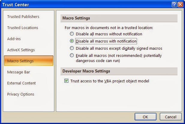
Open up the Trust Center dialog window by clicking the macro security button on the developer tab or press (Alt+LAS) on your keyboard.
The Macro settings tab on trust center dialog window has additional option buttons you can select to change macro level security.
Disable all macros without notification - Select this option when you don't want to run all macros from unknown sources and untrusted publisher's location.
Disable all macros with notification (Default) - Select this option when you want to manage and check its trustworthiness before running the macro.
If you have this option enabled, you just have to click the Options button of every security warning and select the Enable Content option button.
Disable all macros except digitally signed macros - Select this option if you want to automatically run trustworthy digitally signed macros without raising notification.
Enable all macros (not recommend potentially dangerous code can run) - Selecting this option is totally at your own risk, malicious codes can freely run and may cause damage to your system.
This Ultimate Excel Calendar Template allows user, company or any organization to create their own calendars. The template was created in VBA and may require the user to enable macro content in the document.
Annual Calendar Template:
Country - Choose your home country.
Year - Calendar year
First Day of the Week - The first day of the week to be displayed
First Week of The Year - Determines the work week number
The screenshot below shows the calendar of the whole year and the holidays.
The video shows how does Ultimate Excel Calendar template work.
Monthly Calendar Template:
Month - Choose which Month you want to display.
Year - Month year.
First Day of Week - First day of the week to be displayed.
Country - Choose your location
This template will display the Holiday of the Month in the respective dates.
In this example we'll be using three excel functions such as IFERROR, IFand VLOOKUP functions.
=IFERROR(IF(G3="","",VLOOKUP(G3,Sheet1!B:C,2,FALSE)), "No Match Found")
For this example, we'll use the above formula at Cell "G4":
Initially, the formula says that if the value of G3 is blank then set the value of G4 to blank. Otherwise, look for the lookup value (ID) in the table array and return the exact match in the second column (Name) . If the value is not found in the array then return a message to the user.
IFERROR('Formula to Evaluate', value-if-error) - Returns the specified value "No Match Found" if the formula evaluated returns an error value.
IF(logical_test, [value_if_true], [value_if_false]) -Logic test is a comparison between two values (G3=""), test's if the value of G3 is empty. Followed by two arguments which are the value_if_true and value_if_false. If the value of G3 is equal to blank then do nothing or set the Cell's value to blank. While, if the value if G3 is not equal to blank then evaluate the next function.
VLOOKUP(lookup_value, table_array, col_index_num, [range_lookup]) - Looks up the value of G3 in the table array Sheet1!B:C and return the value of the exact match from the column 2.
The following example will give you an idea on how to use VLOOKUP in Microsoft Excel. If you're working with an excel database and want it to be dynamic the VLOOKUP/HLOOKUP functions are very useful for you. The VLOOKUP function looks up value in columns while HLOOKUP does in rows.
This example has two sheets "Price_List" and "Orders" for mobile brands. *Note: The values given are not the actual market prices.
The "Price_List" sheet has three columns ID, Model and Price. This is where we'll be looking up the prices value for every orders made.
Now, on the orders tab we have 3 orders made. We'll add the VLOOKUP function in the Total Price formula. This formula "=VLOOKUP(B2,Price_List!B1:C7,2,FALSE)" will LOOKUP for the price of the unit brand in the Price_List Sheet.
The formula above is a logical condition to calculate the Total Price when the quantity is entered. The condition is:
If the quantity "C2" is blank then it will just lookup the unit price from the Price_List Sheet. And if the quantity is entered it will calculate by multiplying the unit price with the quantity value.


